library(sjmisc)
data(efc)
# linear fit. loess-smoothed line indicates a more
# or less cubic curve
sjp.poly(efc$c160age, efc$quol_5, 1)
## Polynomial degrees: 1
## ---------------------
## p(x^1): 0.000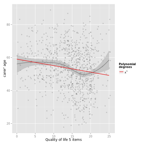
# quadratic fit
sjp.poly(efc$c160age, efc$quol_5, 2)
## Polynomial degrees: 2
## ---------------------
## p(x^1): 0.078
## p(x^2): 0.533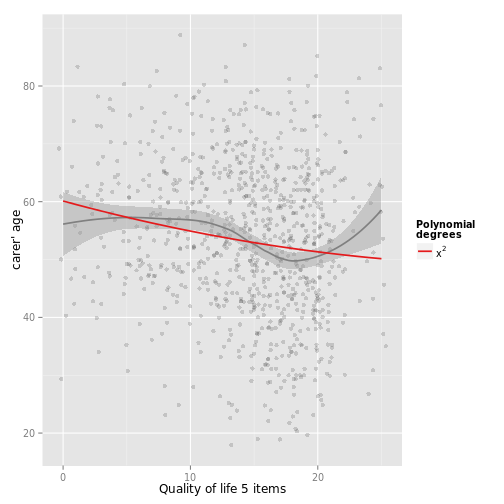
# linear to cubic fit
sjp.poly(efc$c160age, efc$quol_5,
1:4, showScatterPlot = FALSE)## Polynomial degrees: 1
## ---------------------
## p(x^1): 0.000
##
## Polynomial degrees: 2
## ---------------------
## p(x^1): 0.078
## p(x^2): 0.533
##
## Polynomial degrees: 3
## ---------------------
## p(x^1): 0.012
## p(x^2): 0.001
## p(x^3): 0.000
##
## Polynomial degrees: 4
## ---------------------
## p(x^1): 0.777
## p(x^2): 0.913
## p(x^3): 0.505
## p(x^4): 0.254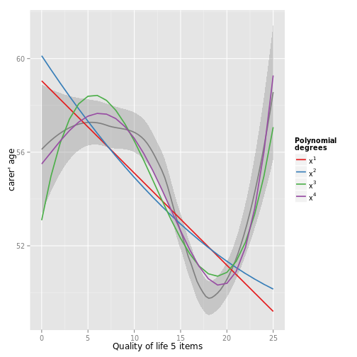
library(sjmisc)
data(efc)
# fit sample model
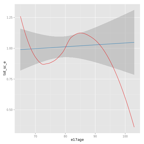
fit <- lm(tot_sc_e ~ c12hour + e17age + e42dep, data = efc)
# inspect relationship between predictors and response
sjp.lm(fit, type = "pred",
showLoess = TRUE, showScatterPlot = FALSE)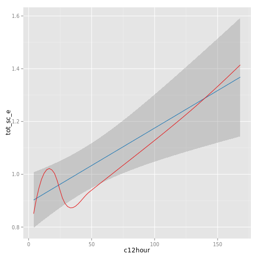
## Warning in simpleLoess(y, x, w, span, degree, parametric, drop.square,
## normalize, : pseudoinverse used at 4.015
## Warning in simpleLoess(y, x, w, span, degree, parametric, drop.square,
## normalize, : neighborhood radius 2.015## Warning in simpleLoess(y, x, w, span, degree, parametric, drop.square,
## normalize, : reciprocal condition number 2.8666e-15## Warning in simpleLoess(y, x, w, span, degree, parametric, drop.square,
## normalize, : There are other near singularities as well. 1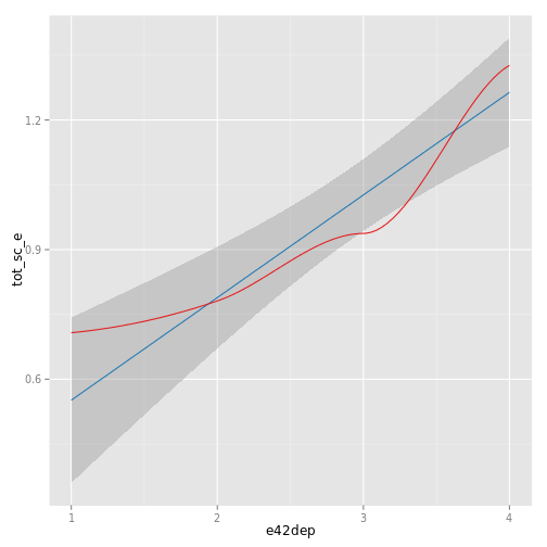
# "e17age" does not seem to be linear correlated to response
# try to find appropiate polynomial. Grey line (loess smoothed)
# indicates best fit. Looks like x^4 has the best fit,
# however, only x^3 has significant p-values.
sjp.poly(fit, "e17age", 2:4, showScatterPlot = FALSE)
## Polynomial degrees: 2
## ---------------------
## p(x^1): 0.734
## p(x^2): 0.721
##
## Polynomial degrees: 3
## ---------------------
## p(x^1): 0.010
## p(x^2): 0.011
## p(x^3): 0.011
##
## Polynomial degrees: 4
## ---------------------
## p(x^1): 0.234
## p(x^2): 0.267
## p(x^3): 0.303
## p(x^4): 0.343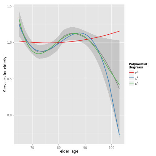
## Not run:
##D # fit new model
##D fit <- lm(tot_sc_e ~ c12hour + e42dep +
##D           e17age + I(e17age^2) + I(e17age^3),
##D           data = efc)
##D # plot marginal effects of polynomial term
##D sjp.lm(fit, type = "poly", poly.term = "e17age")
## End(Not run)