Plot PCA results

# randomly create data frame with 7 items, each consisting of 4 categories
likert_4 <- data.frame(sample(1:4,
                              500,
                              replace = TRUE,
                              prob = c(0.2, 0.3, 0.1, 0.4)),
                       sample(1:4,
                              500,
                              replace = TRUE,
                              prob = c(0.5, 0.25, 0.15, 0.1)),
                       sample(1:4,
                              500,
                              replace = TRUE,
                              prob = c(0.4, 0.15, 0.25, 0.2)),
                       sample(1:4,
                              500,
                              replace = TRUE,
                              prob = c(0.25, 0.1, 0.4, 0.25)),
                       sample(1:4,
                              500,
                              replace = TRUE,
                              prob = c(0.1, 0.4, 0.4, 0.1)),
                       sample(1:4,
                              500,
                              replace = TRUE),
                       sample(1:4,
                              500,
                              replace = TRUE,
                              prob = c(0.35, 0.25, 0.15, 0.25)))

# Create variable labels
colnames(likert_4) <- c("V1", "V2", "V3", "V4", "V5", "V6", "V7")

# plot results from PCA as square-tiled "heatmap"
sjp.pca(likert_4, type = "tile")

## Following items have been removed:
## none.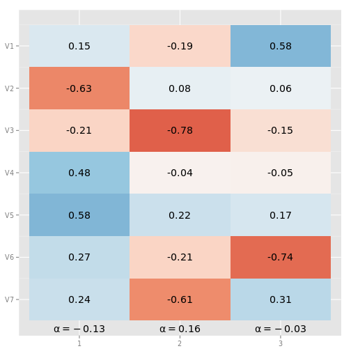

plot of chunk sjp.pca

# plot results from PCA as bars
sjp.pca(likert_4, type = "bar")

## Following items have been removed:
## none.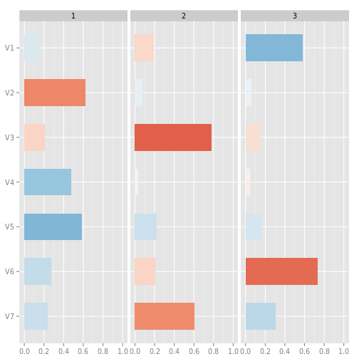

plot of chunk sjp.pca

# manually compute PCA
pca <- prcomp(na.omit(likert_4),
              retx = TRUE,
              center = TRUE,
              scale. = TRUE)
# plot results from PCA as circles, including Eigenvalue-diagnostic.
# note that this plot does not compute the Cronbach's Alpha
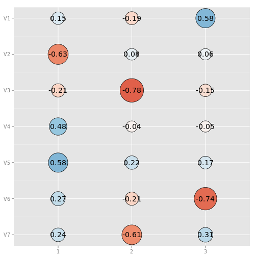
sjp.pca(pca,
        plotEigenvalues = TRUE,
        type = "circle",
        geom.size = 10)

## --------------------------------------------

## Importance of components:
##                           PC1    PC2    PC3    PC4    PC5    PC6
## Standard deviation     1.0775 1.0538 1.0106 0.9964 0.9893 0.9568
## Proportion of Variance 0.1659 0.1587 0.1459 0.1418 0.1398 0.1308
## Cumulative Proportion  0.1659 0.3245 0.4704 0.6122 0.7520 0.8828
##                           PC7
## Standard deviation     0.9056
## Proportion of Variance 0.1172
## Cumulative Proportion  1.0000

## Eigenvalues:

## [1] 1.1610157 1.1105759 1.0212199 0.9928274 0.9787121 0.9154892
## [7] 0.8201599

## --------------------------------------------
## Cronbach's Alpha can only be calculated when having a data frame with each component / variable as column.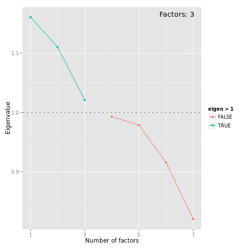

plot of chunk sjp.pca

# -------------------------------
# Data from the EUROFAMCARE sample dataset
# -------------------------------
library(sjmisc)
data(efc)

# retrieve variable and value labels
varlabs <- get_label(efc)

# recveive first item of COPE-index scale
start <- which(colnames(efc) == "c82cop1")
# recveive last item of COPE-index scale
end <- which(colnames(efc) == "c90cop9")

# create data frame with COPE-index scale
mydf <- data.frame(efc[, c(start:end)])
colnames(mydf) <- varlabs[c(start:end)]

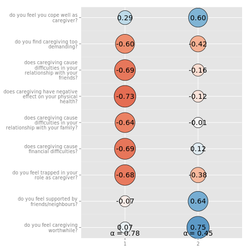
sjp.pca(mydf)

## Following items have been removed:
## none.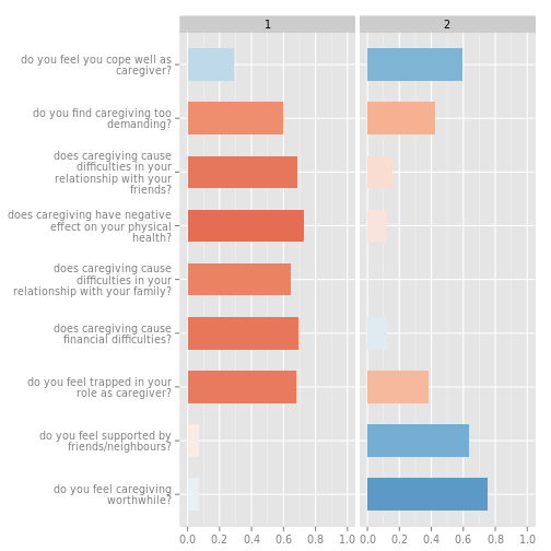

plot of chunk sjp.pca

sjp.pca(mydf, type = "tile")

## Following items have been removed:
## none.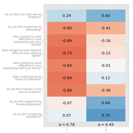

plot of chunk sjp.pca

# -------------------------------
# auto-detection of labels
# -------------------------------
sjp.pca(efc[, c(start:end)], type = "circle", geom.size = 10)

## Following items have been removed:
## none.

plot of chunk sjp.pca