Plot estimates or predicted values of linear models

# --------------------------------------------------
# plotting estimates of linear models as forest plot
# --------------------------------------------------
# fit linear model
fit <- lm(airquality$Ozone ~ airquality$Wind + airquality$Temp + airquality$Solar.R)

# plot estimates with CI
sjp.lm(fit, gridBreaksAt = 2)

# plot estimates with CI
# and with narrower tick marks
# (because "gridBreaksAt" was not specified)
sjp.lm(fit)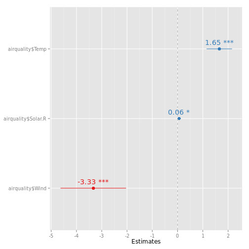

# ---------------------------------------------------
# plotting regression line of linear model (done
# automatically if fitted model has only 1 predictor)
# ---------------------------------------------------
library(sjmisc)
data(efc)
# fit model
fit <- lm(neg_c_7 ~ quol_5, data=efc)
# plot regression line with label strings
sjp.lm(fit,
       axisLabels.x = "Quality of life",
       axisLabels.y = "Burden of care",
       showLoess = TRUE)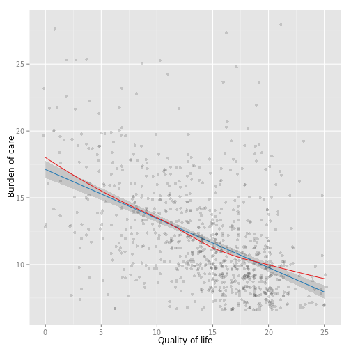

# --------------------------------------------------
# plotting regression lines of each single predictor
# of a fitted model
# --------------------------------------------------
library(sjmisc)
data(efc)
# fit model
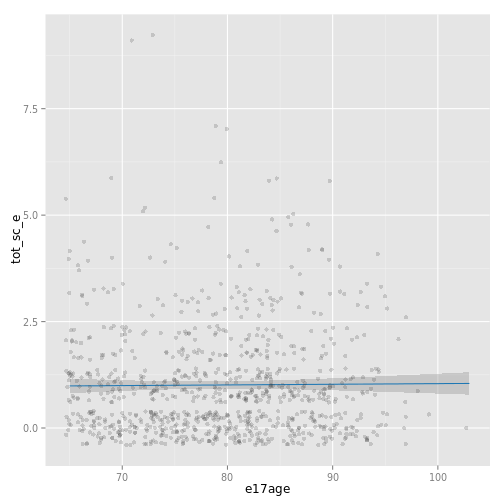
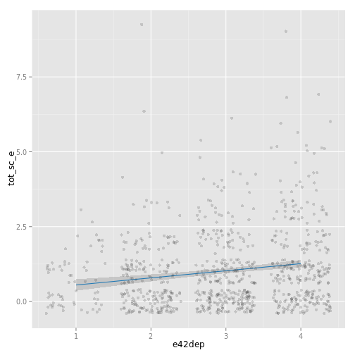
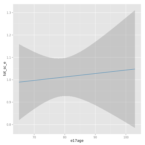
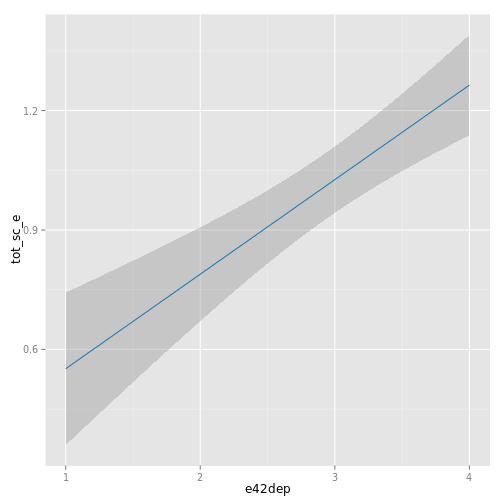
fit <- lm(tot_sc_e ~ c12hour + e17age + e42dep, data=efc)

# reression line and scatter plot
sjp.lm(fit, type = "pred")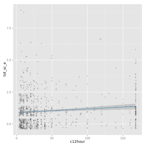

# reression line w/o scatter plot
sjp.lm(fit,
       type = "pred",
       showScatterPlot = FALSE)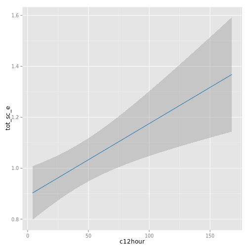

# --------------------------
# plotting model assumptions
# --------------------------
sjp.lm(fit, type = "ma")

## Error: Package 'lmtest' needed for this function to work. Please install it.

## Not run: 
##D # --------------------------
##D # plotting polynomial terms
##D # --------------------------
##D library(sjmisc)
##D data(efc)
##D # fit sample model
##D fit <- lm(tot_sc_e ~ c12hour + e17age + e42dep, data = efc)
##D # "e17age" does not seem to be linear correlated to response
##D # try to find appropiate polynomial. Grey line (loess smoothed)
##D # indicates best fit. Looks like x^3 has a good fit.
##D # (not checked for significance yet).
##D sjp.poly(fit, "e17age", 2:4, showScatterPlot = FALSE)
##D # fit new model
##D fit <- lm(tot_sc_e ~ c12hour + e42dep +
##D           e17age + I(e17age^2) + I(e17age^3),
##D           data = efc)
##D # plot marginal effects of polynomial term
##D sjp.lm(fit, type = "poly", poly.term = "e17age")
##D 
##D 
##D library(splines)
##D # fit new model with "splines"-package, "bs"
##D fit <- lm(tot_sc_e ~ c12hour + e42dep + bs(e17age, 3), data = efc)
##D # plot marginal effects of polynomial term, same call as above
##D sjp.lm(fit, type = "poly", poly.term = "e17age")
## End(Not run)