### Using granovagg.ds to examine trends or effects for repeated measures data.

# This example corresponds to case 1b in Pruzek and Helmreich (2009). In this
# graphic we're looking for the effect of treatment on patients with anorexia.

data(anorexia.sub)
granovagg.ds(anorexia.sub,
             revc = TRUE,
             main = "Assessment Plot for weights to assess\
                     Family Therapy treatment for Anorexia Patients",
             xlab = "Weight after therapy (lbs.)",
             ylab = "Weight before therapy (lbs.)"
)
## Summary Statistics
## n 17.000
## Postwt mean 90.494
## Prewt mean 83.229
## mean(D = Postwt - Prewt) 7.265
## SD(D) 7.157
## Effect Size 1.015
## r(Postwt, Prewt) 0.538
## r(Postwt + Prewt, D) 0.546
## Lower 95% Confidence Interval 3.585
## Upper 95% Confidence Interval 10.945
## t (D-bar) 4.185
## df.t 16.000
## p-value (t-statistic) 0.001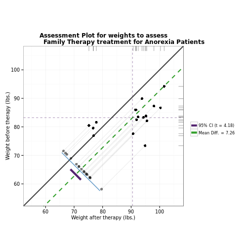
### Using granovagg.ds to compare two experimental treatments (with blocking)

# This example corresponds to case 2a in Pruzek and Helmreich (2009). For this
# data, we're comparing the effects of two different virus preparations on the
# number of lesions produced on a tobacco leaf.

data(tobacco)
granovagg.ds(tobacco[, c("prep1", "prep2")],
             main = "Local Lesions on Tobacco Leaves",
             xlab = "Virus Preparation 1",
             ylab = "Virus Preparation 2"
)
## Summary Statistics
## n 8.000
## prep1 mean 15.000
## prep2 mean 11.000
## mean(D = prep1 - prep2) 4.000
## SD(D) 4.309
## Effect Size 0.928
## r(prep1, prep2) 0.899
## r(prep1 + prep2, D) 0.766
## Lower 95% Confidence Interval 0.397
## Upper 95% Confidence Interval 7.603
## t (D-bar) 2.625
## df.t 7.000
## p-value (t-statistic) 0.034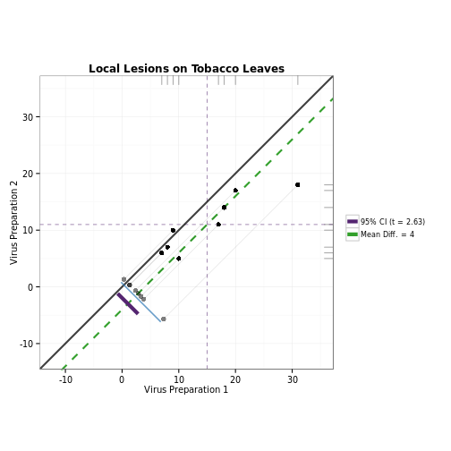
### Using granovagg.ds to compare two experimental treatments (with blocking)

# This example corresponds to case 2a in Pruzek and Helmreich (2009). For this
# data, we're comparing the wear resistance of two different shoe sole
# materials, each randomly assigned to the feet of 10 boys.

library(MASS) # Contains the shoes dataset
shoes <- as.data.frame(shoes)
granovagg.ds(shoes,
             revc = TRUE,
             main = "Shoe Wear",
             xlab = "Sole Material B",
             ylab = "Sole Material A",
)
## Summary Statistics
## n 10.000
## B mean 11.040
## A mean 10.630
## mean(D = B - A) 0.410
## SD(D) 0.387
## Effect Size 1.059
## r(B, A) 0.988
## r(B + A, D) 0.174
## Lower 95% Confidence Interval 0.133
## Upper 95% Confidence Interval 0.687
## t (D-bar) 3.349
## df.t 9.000
## p-value (t-statistic) 0.009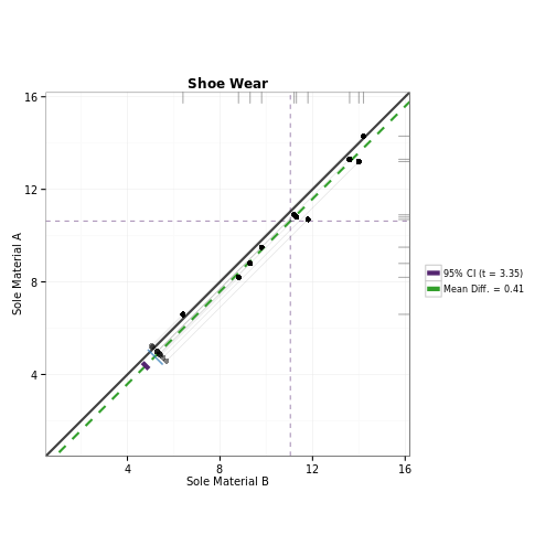
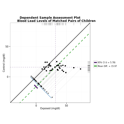
### Using granovagg.ds to compare matched individuals for two treatments

# This example corresponds to case 2b in Pruzek and Helmreich (2009). For this
# data, we're examining the level of lead (in mg/dl) present in the blood of
# children. Children of parents who had worked in a factory where lead was used
# in making batteries were matched by age, exposure to traffic, and neighborhood
# with children whose parents did not work in lead-related industries.

data(blood_lead)
granovagg.ds(blood_lead,
             sw = .1,
             main = "Dependent Sample Assessment Plot
             Blood Lead Levels of Matched Pairs of Children",
             xlab = "Exposed (mg/dl)",
             ylab = "Control (mg/dl)"
)
## Summary Statistics
## n 33.000
## Exposed mean 31.848
## Control mean 15.879
## mean(D = Exposed - Control) 15.970
## SD(D) 15.864
## Effect Size 1.007
## r(Exposed, Control) -0.179
## r(Exposed + Control, D) 0.824
## Lower 95% Confidence Interval 10.345
## Upper 95% Confidence Interval 21.595
## t (D-bar) 5.783
## df.t 32.000
## p-value (t-statistic) 0.000