data(arousal)
contrasts22 <- data.frame( c(-.5,-.5,.5,.5),
  c(-.5,.5,-.5,.5), c(.5,-.5,-.5,.5) )
names(contrasts22) <- c("Drug.A", "Drug.B", "Drug.A.B")
granovagg.contr(arousal, contrasts = contrasts22)
## No id variables; using all as measure variables
##
## Linear Model Summary##
## Call:
## lm(formula = Response ~ Contrast)
##
## Residuals:
## Min 1Q Median 3Q Max
## -5.910 -2.015 -0.075 1.885 6.290
##
## Coefficients:
## Estimate Std. Error t value Pr(>|t|)
## (Intercept) 24.0825 0.4657 51.712 < 2e-16 ***
## Contrast1 3.4650 0.9314 3.720 0.000676 ***
## Contrast2 3.9150 0.9314 4.203 0.000166 ***
## Contrast3 0.0750 0.9314 0.081 0.936267
## ---
## Signif. codes: 0 '***' 0.001 '**' 0.01 '*' 0.05 '.' 0.1 ' ' 1
##
## Residual standard error: 2.945 on 36 degrees of freedom
## Multiple R-squared: 0.4668, Adjusted R-squared: 0.4223
## F-statistic: 10.5 on 3 and 36 DF, p-value: 4.173e-05##
## (Weighted) means, mean differences, and standardized effect size## neg pos diff stEftSze
## Contrast1 22.4 25.8 3.465 1.1764
## Contrast2 22.1 26.0 3.915 1.3292
## Contrast3 24.0 24.1 0.075 0.0255##
## Summary statistics by group## group group.mean standard.deviation pooled.standard.deviation
## 1 1 20.43 2.414 2.945
## 2 2 24.27 2.809 2.945
## 3 3 23.82 2.738 2.945
## 4 4 27.81 3.672 2.945##
## The contrasts you specified## Drug.A Drug.B Drug.A.B
## [1,] -0.5 -0.5 0.5
## [2,] -0.5 0.5 -0.5
## [3,] 0.5 -0.5 -0.5
## [4,] 0.5 0.5 0.5## Since you elected to print four plots per page
## granovagg.contr won't return any plot objects.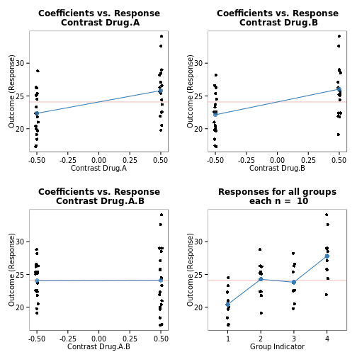
## NULLdata(rat)
dat6 <- matrix(c(1, 1, 1, -1, -1, -1, -1, 1, 0, -1, 1, 0, 1, 1, -2,
1, 1, -2, -1, 1, 0, 1, -1, 0, 1, 1, -2, -1, -1, 2), ncol = 5)
granovagg.contr(rat[,1], contrasts = dat6, ylab = "Rat Weight Gain",
xlab = c("Amount 1 vs. Amount 2", "Type 1 vs. Type 2",
"Type 1 & 2 vs Type 3", "Interaction of Amount and Type 1 & 2",
"Interaction of Amount and Type (1, 2), 3"))## No id variables; using all as measure variables
##
## Linear Model Summary##
## Call:
## lm(formula = Response ~ Contrast)
##
## Residuals:
## Min 1Q Median 3Q Max
## -29.90 -8.75 2.20 10.80 27.30
##
## Coefficients:
## Estimate Std. Error t value Pr(>|t|)
## (Intercept) 8.787e+01 1.891e+00 46.465 < 2e-16 ***
## Contrast1 2.202e+01 5.730e+00 3.843 0.000322 ***
## Contrast2 -5.000e-01 4.632e+00 -0.108 0.914440
## Contrast3 5.933e+00 5.349e+00 1.109 0.272205
## Contrast4 2.547e-15 4.632e+00 0.000 1.000000
## Contrast5 1.253e+01 5.349e+00 2.343 0.022827 *
## ---
## Signif. codes: 0 '***' 0.001 '**' 0.01 '*' 0.05 '.' 0.1 ' ' 1
##
## Residual standard error: 14.65 on 54 degrees of freedom
## Multiple R-squared: 0.2848, Adjusted R-squared: 0.2185
## F-statistic: 4.3 on 5 and 54 DF, p-value: 0.002299##
## (Weighted) means, mean differences, and standardized effect size## neg pos diff stEftSze
## Contrast1 80.6 95.1 14.53 0.9922
## Contrast2 89.6 89.1 -0.50 -0.0341
## Contrast3 84.9 89.3 4.45 0.3038
## Contrast4 89.3 89.3 0.00 0.0000
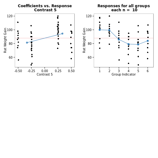
## Contrast5 81.3 94.5 13.20 0.9012##
## Summary statistics by group## group group.mean standard.deviation pooled.standard.deviation
## 1 1 100.0 15.14 14.65
## 2 2 99.5 10.92 14.65
## 3 3 85.9 15.02 14.65
## 4 4 79.2 13.89 14.65
## 5 5 78.7 16.55 14.65
## 6 6 83.9 15.71 14.65##
## The contrasts you specified## [,1] [,2] [,3] [,4] [,5]
## [1,] 1 -1 1 -1 1
## [2,] 1 1 1 1 1
## [3,] 1 0 -2 0 -2
## [4,] -1 -1 1 1 -1
## [5,] -1 1 1 -1 -1
## [6,] -1 0 -2 0 2## Since you elected to print four plots per page
## granovagg.contr won't return any plot objects.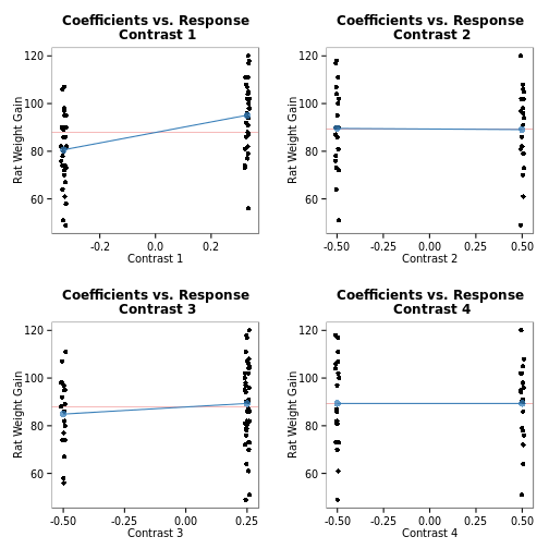
## NULL#Polynomial Contrasts
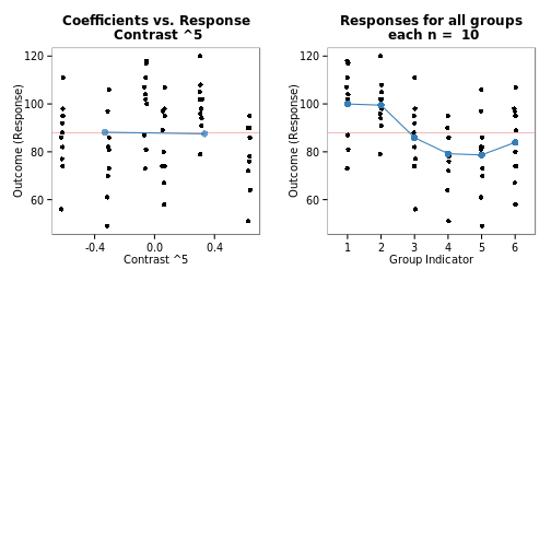
granovagg.contr(rat[,1],contrasts = contr.poly(6))## No id variables; using all as measure variables
##
## Linear Model Summary##
## Call:
## lm(formula = Response ~ Contrast)
##
## Residuals:
## Min 1Q Median 3Q Max
## -29.90 -8.75 2.20 10.80 27.30
##
## Coefficients:
## Estimate Std. Error t value Pr(>|t|)
## (Intercept) 87.864 1.891 46.464 < 2e-16 ***
## Contrast1 -19.135 4.968 -3.851 0.000314 ***
## Contrast2 9.669 5.054 1.913 0.061050 .
## Contrast3 8.339 5.519 1.511 0.136643
## Contrast4 -4.405 5.260 -0.837 0.406018
## Contrast5 1.343 4.678 0.287 0.775079
## ---
## Signif. codes: 0 '***' 0.001 '**' 0.01 '*' 0.05 '.' 0.1 ' ' 1
##
## Residual standard error: 14.65 on 54 degrees of freedom
## Multiple R-squared: 0.2848, Adjusted R-squared: 0.2185
## F-statistic: 4.3 on 5 and 54 DF, p-value: 0.002299##
## (Weighted) means, mean differences, and standardized effect size## neg pos diff stEftSze
## Contrast1 95.1 80.6 -14.533 -0.9922
## Contrast2 85.8 92.0 6.125 0.4182
## Contrast3 86.0 89.8 3.800 0.2594
## Contrast4 89.1 87.2 -1.850 -0.1263
## Contrast5 88.2 87.5 -0.667 -0.0455##
## Summary statistics by group## group group.mean standard.deviation pooled.standard.deviation
## 1 1 100.0 15.14 14.65
## 2 2 99.5 10.92 14.65
## 3 3 85.9 15.02 14.65
## 4 4 79.2 13.89 14.65
## 5 5 78.7 16.55 14.65
## 6 6 83.9 15.71 14.65##
## The contrasts you specified## .L .Q .C ^4 ^5
## [1,] -0.598 0.546 -0.373 0.189 -0.063
## [2,] -0.359 -0.109 0.522 -0.567 0.315
## [3,] -0.120 -0.436 0.298 0.378 -0.630
## [4,] 0.120 -0.436 -0.298 0.378 0.630
## [5,] 0.359 -0.109 -0.522 -0.567 -0.315
## [6,] 0.598 0.546 0.373 0.189 0.063## Since you elected to print four plots per page
## granovagg.contr won't return any plot objects.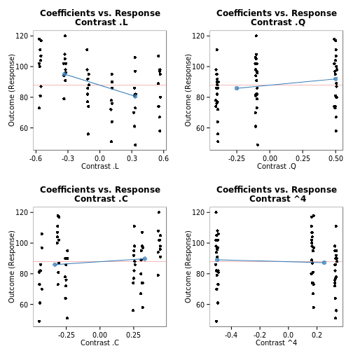
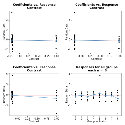
## NULL#based on random data
data.random <- rt(64, 5)
granovagg.contr(data.random, contrasts = contr.helmert(8),
ylab = "Random Data")## No id variables; using all as measure variables
##
## Linear Model Summary##
## Call:
## lm(formula = Response ~ Contrast)
##
## Residuals:
## Min 1Q Median 3Q Max
## -4.3820 -0.5528 0.0547 0.5552 5.1854
##
## Coefficients:
## Estimate Std. Error t value Pr(>|t|)
## (Intercept) -0.2822 0.1656 -1.704 0.0940 .
## Contrast1 0.1229 0.3313 0.371 0.7120
## Contrast2 -0.1388 0.3835 -0.362 0.7187
## Contrast3 0.2475 0.4049 0.611 0.5434
## Contrast4 0.5108 0.4197 1.217 0.2286
## Contrast5 -0.1296 0.4277 -0.303 0.7630
## Contrast6 -0.1215 0.4332 -0.281 0.7801
## Contrast7 -0.7683 0.4378 -1.755 0.0847 .
## ---
## Signif. codes: 0 '***' 0.001 '**' 0.01 '*' 0.05 '.' 0.1 ' ' 1
##
## Residual standard error: 1.325 on 56 degrees of freedom
## Multiple R-squared: 0.08768, Adjusted R-squared: -0.02636
## F-statistic: 0.7688 on 7 and 56 DF, p-value: 0.6157##
## (Weighted) means, mean differences, and standardized effect size## neg pos diff stEftSze
## Contrast1 -0.389 -0.14332 0.246 0.185
## Contrast2 -0.266 -0.47390 -0.208 -0.157
## Contrast3 -0.335 -0.00435 0.331 0.250
## Contrast4 -0.253 0.38561 0.638 0.482
## Contrast5 -0.125 -0.28073 -0.156 -0.118
## Contrast6 -0.151 -0.29309 -0.142 -0.107
## Contrast7 -0.171 -1.05054 -0.879 -0.664##
## Summary statistics by group## group group.mean standard.deviation pooled.standard.deviation
## 1 1 -0.389113 1.2740 1.325
## 2 2 -0.143321 0.6319 1.325
## 3 3 -0.473900 0.8075 1.325
## 4 4 -0.004354 0.7276 1.325
## 5 5 0.385610 2.2285 1.325
## 6 6 -0.280731 1.0760 1.325
## 7 7 -0.293095 0.7453 1.325
## 8 8 -1.050537 2.0402 1.325##
## The contrasts you specified## [,1] [,2] [,3] [,4] [,5] [,6] [,7]
## 1 -1 -1 -1 -1 -1 -1 -1
## 2 1 -1 -1 -1 -1 -1 -1
## 3 0 2 -1 -1 -1 -1 -1
## 4 0 0 3 -1 -1 -1 -1
## 5 0 0 0 4 -1 -1 -1
## 6 0 0 0 0 5 -1 -1
## 7 0 0 0 0 0 6 -1
## 8 0 0 0 0 0 0 7## Since you elected to print four plots per page
## granovagg.contr won't return any plot objects.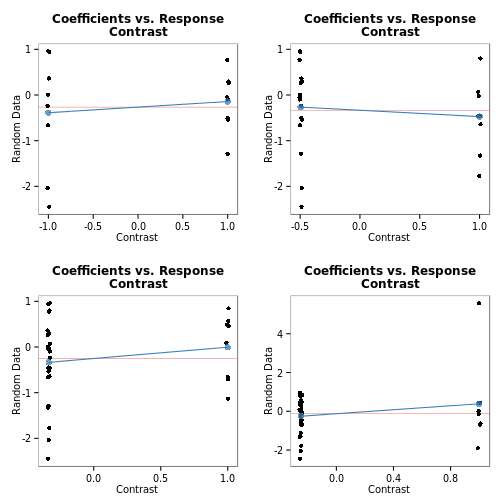
## NULL