data(arousal)
#Drug A
granovagg.1w(arousal[,1:2], h.rng = 1.6, v.rng = 0.5)
##
## By-group summary statistics for your input data (ordered by group means)## group group.mean trimmed.mean contrast variance
## 1 Placebo 20.43 20.30 -1.92 5.83
## 2 Drug.A 24.27 24.45 1.92 7.89
## standard.deviation group.size
## 1 2.41 10
## 2 2.81 10##
## Below is a t-test summary of your input data##
## Two Sample t-test
##
## data: unstacked.data[, 1] and unstacked.data[, 2]
## t = -3.2786, df = 18, p-value = 0.004174
## alternative hypothesis: true difference in means is not equal to 0
## 95 percent confidence interval:
## -6.300681 -1.379319
## sample estimates:
## mean of x mean of y
## 20.43 24.27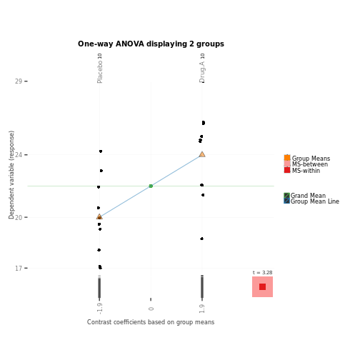
###

library(MASS) # Contains the anorexia dataset
wt.gain <- anorexia[, 3] - anorexia[, 2]
granovagg.1w(wt.gain, group = anorexia[, 1])
##
## By-group summary statistics for your input data (ordered by group means)## group group.mean trimmed.mean contrast variance standard.deviation
## 2 Cont -0.45 -1.16 -3.21 63.82 7.99
## 1 CBT 3.01 1.80 0.24 53.41 7.31
## 3 FT 7.26 7.91 4.50 51.23 7.16
## group.size
## 2 26
## 1 29
## 3 17##
## Below is a linear model summary of your input data##
## Call:
## lm(formula = score ~ group, data = owp$data)
##
## Residuals:
## Min 1Q Median 3Q Max
## -12.565 -4.543 -1.007 3.846 17.893
##
## Coefficients:
## Estimate Std. Error t value Pr(>|t|)
## (Intercept) 3.007 1.398 2.151 0.0350 *
## groupCont -3.457 2.033 -1.700 0.0936 .
## groupFT 4.258 2.300 1.852 0.0684 .
## ---
## Signif. codes: 0 '***' 0.001 '**' 0.01 '*' 0.05 '.' 0.1 ' ' 1
##
## Residual standard error: 7.528 on 69 degrees of freedom
## Multiple R-squared: 0.1358, Adjusted R-squared: 0.1108
## F-statistic: 5.422 on 2 and 69 DF, p-value: 0.006499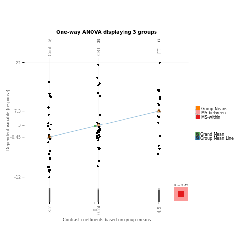
###

data(poison)
##Note violation of constant variance across groups in following graphic.
granovagg.1w(poison$SurvTime, group = poison$Group, ylab = "Survival Time")
##
## By-group summary statistics for your input data (ordered by group means)## group group.mean trimmed.mean contrast variance standard.deviation
## 3 3 0.21 0.21 -0.27 0.00 0.02
## 9 9 0.24 0.24 -0.24 0.00 0.01
## 2 2 0.32 0.32 -0.16 0.01 0.08
## 12 12 0.32 0.32 -0.15 0.00 0.03
## 6 6 0.34 0.34 -0.14 0.00 0.05
## 8 8 0.38 0.38 -0.10 0.00 0.06
## 1 1 0.41 0.41 -0.07 0.00 0.07
## 7 7 0.57 0.57 0.09 0.02 0.16
## 10 10 0.61 0.61 0.13 0.01 0.11
## 11 11 0.67 0.67 0.19 0.07 0.27
## 5 5 0.82 0.82 0.34 0.11 0.34
## 4 4 0.88 0.88 0.40 0.03 0.16
## group.size
## 3 4
## 9 4
## 2 4
## 12 4
## 6 4
## 8 4
## 1 4
## 7 4
## 10 4
## 11 4
## 5 4
## 4 4##
## The following groups are likely to be overplotted## group group.mean contrast
## 2 2 0.32 -0.16
## 12 12 0.32 -0.15
## 6 6 0.34 -0.14##
## Below is a linear model summary of your input data##
## Call:
## lm(formula = score ~ group, data = owp$data)
##
## Residuals:
## Min 1Q Median 3Q Max
## -0.32500 -0.04875 0.00500 0.04313 0.42500
##
## Coefficients:
## Estimate Std. Error t value Pr(>|t|)
## (Intercept) 0.41250 0.07457 5.532 2.94e-06 ***
## group2 -0.09250 0.10546 -0.877 0.386230
## group3 -0.20250 0.10546 -1.920 0.062781 .
## group4 0.46750 0.10546 4.433 8.37e-05 ***
## group5 0.40250 0.10546 3.817 0.000513 ***
## group6 -0.07750 0.10546 -0.735 0.467163
## group7 0.15500 0.10546 1.470 0.150304
## group8 -0.03750 0.10546 -0.356 0.724219
## group9 -0.17750 0.10546 -1.683 0.101000
## group10 0.19750 0.10546 1.873 0.069235 .
## group11 0.25500 0.10546 2.418 0.020791 *
## group12 -0.08750 0.10546 -0.830 0.412164
## ---
## Signif. codes: 0 '***' 0.001 '**' 0.01 '*' 0.05 '.' 0.1 ' ' 1
##
## Residual standard error: 0.1491 on 36 degrees of freedom
## Multiple R-squared: 0.7335, Adjusted R-squared: 0.6521
## F-statistic: 9.01 on 11 and 36 DF, p-value: 1.986e-07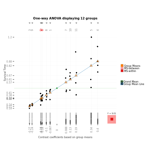
##RateSurvTime = SurvTime^-1
granovagg.1w(poison$RateSurvTime, group = poison$Group,
ylab = "Survival Rate = Inverse of Survival Time")
##
## By-group summary statistics for your input data (ordered by group means)## group group.mean trimmed.mean contrast variance standard.deviation
## 4 4 1.16 1.16 -1.46 0.04 0.20
## 5 5 1.39 1.39 -1.23 0.31 0.55
## 10 10 1.69 1.69 -0.93 0.13 0.36
## 11 11 1.70 1.70 -0.92 0.49 0.70
## 7 7 1.86 1.86 -0.76 0.24 0.49
## 1 1 2.49 2.49 -0.14 0.25 0.50
## 8 8 2.71 2.71 0.09 0.17 0.42
## 6 6 3.03 3.03 0.41 0.18 0.42
## 12 12 3.09 3.09 0.47 0.06 0.24
## 2 2 3.27 3.27 0.65 0.68 0.82
## 9 9 4.26 4.26 1.64 0.06 0.23
## 3 3 4.80 4.80 2.18 0.28 0.53
## group.size
## 4 4
## 5 4
## 10 4
## 11 4
## 7 4
## 1 4
## 8 4
## 6 4
## 12 4
## 2 4
## 9 4
## 3 4##
## The following groups are likely to be overplotted## group group.mean contrast
## 10 10 1.69 -0.93
## 11 11 1.70 -0.92
## 6 6 3.03 0.41
## 12 12 3.09 0.47##
## Below is a linear model summary of your input data##
## Call:
## lm(formula = score ~ group, data = owp$data)
##
## Residuals:
## Min 1Q Median 3Q Max
## -0.76848 -0.29639 -0.06915 0.25455 1.07932
##
## Coefficients:
## Estimate Std. Error t value Pr(>|t|)
## (Intercept) 2.4869 0.2450 10.151 4.16e-12 ***
## group2 0.7816 0.3465 2.256 0.030247 *
## group3 2.3158 0.3465 6.684 8.56e-08 ***
## group4 -1.3234 0.3465 -3.820 0.000508 ***
## group5 -1.0935 0.3465 -3.156 0.003226 **
## group6 0.5421 0.3465 1.565 0.126414
## group7 -0.6242 0.3465 -1.801 0.080010 .
## group8 0.2270 0.3465 0.655 0.516468
## group9 1.7781 0.3465 5.132 1.00e-05 ***
## group10 -0.7972 0.3465 -2.301 0.027299 *
## group11 -0.7853 0.3465 -2.267 0.029517 *
## group12 0.6049 0.3465 1.746 0.089344 .
## ---
## Signif. codes: 0 '***' 0.001 '**' 0.01 '*' 0.05 '.' 0.1 ' ' 1
##
## Residual standard error: 0.49 on 36 degrees of freedom
## Multiple R-squared: 0.8681, Adjusted R-squared: 0.8277
## F-statistic: 21.53 on 11 and 36 DF, p-value: 1.289e-12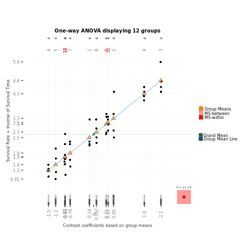
##Nonparametric version: RateSurvTime ranked and rescaled
##to be comparable to RateSurvTime;
##note labels as well as residual (rug) plot below.
granovagg.1w(poison$RankRateSurvTime, group = poison$Group,
ylab = "Ranked and Centered Survival Rates",
main = "One-way ANOVA display, poison data (ignoring 2-way set-up)",
res = TRUE)
##
## By-group summary statistics for your input data (ordered by group means)## group group.mean trimmed.mean contrast variance standard.deviation
## 4 4 1.11 1.11 -1.38 0.03 0.18
## 5 5 1.36 1.36 -1.13 0.28 0.53
## 10 10 1.67 1.67 -0.82 0.10 0.31
## 11 11 1.69 1.69 -0.80 0.50 0.71
## 7 7 1.82 1.82 -0.67 0.24 0.49
## 1 1 2.39 2.39 -0.10 0.30 0.55
## 8 8 2.72 2.72 0.23 0.19 0.44
## 6 6 3.04 3.04 0.55 0.18 0.42
## 12 12 3.09 3.09 0.61 0.05 0.22
## 2 2 3.15 3.15 0.66 0.39 0.62
## 9 9 3.78 3.78 1.29 0.03 0.16
## 3 3 4.04 4.04 1.55 0.03 0.16
## group.size
## 4 4
## 5 4
## 10 4
## 11 4
## 7 4
## 1 4
## 8 4
## 6 4
## 12 4
## 2 4
## 9 4
## 3 4##
## The following groups are likely to be overplotted## group group.mean contrast
## 10 10 1.67 -0.82
## 11 11 1.69 -0.80
## 6 6 3.04 0.55
## 12 12 3.09 0.61
## 2 2 3.15 0.66##
## Below is a linear model summary of your input data##
## Call:
## lm(formula = score ~ group, data = owp$data)
##
## Residuals:
## Min 1Q Median 3Q Max
## -0.7375 -0.2900 -0.0375 0.2606 0.9225
##
## Coefficients:
## Estimate Std. Error t value Pr(>|t|)
## (Intercept) 2.3925 0.2195 10.899 5.93e-13 ***
## group2 0.7550 0.3105 2.432 0.020121 *
## group3 1.6425 0.3105 5.291 6.16e-06 ***
## group4 -1.2825 0.3105 -4.131 0.000205 ***
## group5 -1.0300 0.3105 -3.318 0.002083 **
## group6 0.6475 0.3105 2.086 0.044157 *
## group7 -0.5775 0.3105 -1.860 0.071043 .
## group8 0.3250 0.3105 1.047 0.302141
## group9 1.3900 0.3105 4.477 7.33e-05 ***
## group10 -0.7225 0.3105 -2.327 0.025691 *
## group11 -0.7050 0.3105 -2.271 0.029235 *
## group12 0.7025 0.3105 2.263 0.029775 *
## ---
## Signif. codes: 0 '***' 0.001 '**' 0.01 '*' 0.05 '.' 0.1 ' ' 1
##
## Residual standard error: 0.439 on 36 degrees of freedom
## Multiple R-squared: 0.8542, Adjusted R-squared: 0.8097
## F-statistic: 19.18 on 11 and 36 DF, p-value: 7.233e-12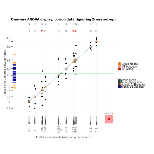
###
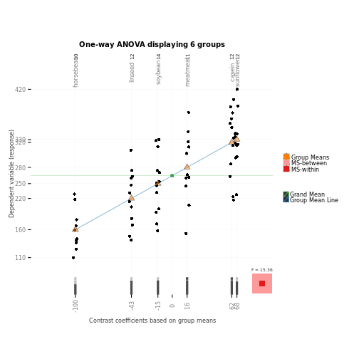
data(chickwts)
?chickwts # An explanation of the chickwts dataset
with(chickwts, granovagg.1w(weight, group = feed)) # Modeling weight as explained by feed type##
## By-group summary statistics for your input data (ordered by group means)## group group.mean trimmed.mean contrast variance
## 2 horsebean 160.20 154.33 -101.11 1491.96
## 3 linseed 218.75 219.50 -42.56 2728.57
## 5 soybean 246.43 246.50 -14.88 2929.96
## 4 meatmeal 276.91 280.43 15.60 4212.09
## 1 casein 323.58 331.38 62.27 4151.72
## 6 sunflower 328.92 326.38 67.61 2384.99
## standard.deviation group.size
## 2 38.63 10
## 3 52.24 12
## 5 54.13 14
## 4 64.90 11
## 1 64.43 12
## 6 48.84 12##
## Below is a linear model summary of your input data##
## Call:
## lm(formula = score ~ group, data = owp$data)
##
## Residuals:
## Min 1Q Median 3Q Max
## -123.909 -34.413 1.571 38.170 103.091
##
## Coefficients:
## Estimate Std. Error t value Pr(>|t|)
## (Intercept) 323.583 15.834 20.436 < 2e-16 ***
## grouphorsebean -163.383 23.485 -6.957 2.07e-09 ***
## grouplinseed -104.833 22.393 -4.682 1.49e-05 ***
## groupmeatmeal -46.674 22.896 -2.039 0.045567 *
## groupsoybean -77.155 21.578 -3.576 0.000665 ***
## groupsunflower 5.333 22.393 0.238 0.812495
## ---
## Signif. codes: 0 '***' 0.001 '**' 0.01 '*' 0.05 '.' 0.1 ' ' 1
##
## Residual standard error: 54.85 on 65 degrees of freedom
## Multiple R-squared: 0.5417, Adjusted R-squared: 0.5064
## F-statistic: 15.36 on 5 and 65 DF, p-value: 5.936e-10