# Note that the data sets used in this example may not be perfectly suitable for
# fitting linear models. I just used them because they are part of the R-software.

# fit "dummy" model. Note that moderator should enter
# first the model, followed by predictor. Else, use
# argument "swapPredictors" to change predictor on
# x-axis with moderator
fit <- lm(weight ~ Diet * Time, data = ChickWeight)

# show summary to see significant interactions
summary(fit)
##
## Call:
## lm(formula = weight ~ Diet * Time, data = ChickWeight)
##
## Residuals:
## Min 1Q Median 3Q Max
## -135.425 -13.757 -1.311 11.069 130.391
##
## Coefficients:
## Estimate Std. Error t value Pr(>|t|)
## (Intercept) 30.9310 4.2468 7.283 1.09e-12 ***
## Diet2 -2.2974 7.2672 -0.316 0.75202
## Diet3 -12.6807 7.2672 -1.745 0.08154 .
## Diet4 -0.1389 7.2865 -0.019 0.98480
## Time 6.8418 0.3408 20.076 < 2e-16 ***
## Diet2:Time 1.7673 0.5717 3.092 0.00209 **
## Diet3:Time 4.5811 0.5717 8.014 6.33e-15 ***
## Diet4:Time 2.8726 0.5781 4.969 8.92e-07 ***
## ---
## Signif. codes: 0 '***' 0.001 '**' 0.01 '*' 0.05 '.' 0.1 ' ' 1
##
## Residual standard error: 34.07 on 570 degrees of freedom
## Multiple R-squared: 0.773, Adjusted R-squared: 0.7702
## F-statistic: 277.3 on 7 and 570 DF, p-value: < 2.2e-16# plot regression line of interaction terms, including value labels
sjp.int(fit, type = "eff", showValueLabels = TRUE)## Error: Package 'effects' needed for this function to work. Please install it.# load sample data set
library(sjmisc)
data(efc)
# create data frame with variables that should be included
# in the model
mydf <- data.frame(usage = efc$tot_sc_e,
sex = efc$c161sex,
education = efc$c172code,
burden = efc$neg_c_7,
dependency = efc$e42dep)
# convert gender predictor to factor
mydf$sex <- relevel(factor(mydf$sex), ref = "2")
# fit "dummy" model
fit <- lm(usage ~ .*., data = mydf)
summary(fit)##
## Call:
## lm(formula = usage ~ . * ., data = mydf)
##
## Residuals:
## Min 1Q Median 3Q Max
## -2.4070 -0.8149 -0.2876 0.3931 8.2089
##
## Coefficients:
## Estimate Std. Error t value Pr(>|t|)
## (Intercept) 1.75061 0.71461 2.450 0.0145 *
## sex1 -0.09252 0.47518 -0.195 0.8457
## education -0.30402 0.27913 -1.089 0.2764
## burden -0.08038 0.05468 -1.470 0.1419
## dependency -0.45307 0.21478 -2.109 0.0352 *
## sex1:education -0.04657 0.15463 -0.301 0.7634
## sex1:burden -0.02251 0.02785 -0.808 0.4192
## sex1:dependency 0.16118 0.11559 1.394 0.1636
## education:burden 0.01110 0.01773 0.626 0.5316
## education:dependency 0.13983 0.08095 1.727 0.0845 .
## burden:dependency 0.02880 0.01245 2.314 0.0209 *
## ---
## Signif. codes: 0 '***' 0.001 '**' 0.01 '*' 0.05 '.' 0.1 ' ' 1
##
## Residual standard error: 1.221 on 822 degrees of freedom
## (75 observations deleted due to missingness)
## Multiple R-squared: 0.06001, Adjusted R-squared: 0.04858
## F-statistic: 5.248 on 10 and 822 DF, p-value: 1.661e-07# plot interactions. note that type = "cond" only considers
# significant interactions by default. use "plevel" to
# adjust p-level sensivity
sjp.int(fit, type = "cond")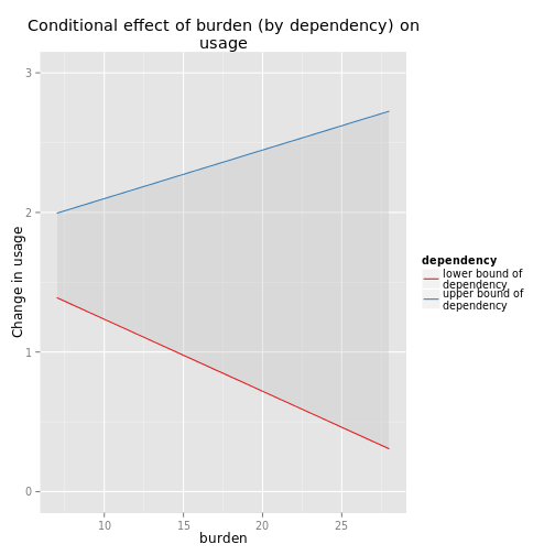
# plot only selected interaction term for
# type = "eff"
sjp.int(fit, type = "eff", int.term = "sex*education")
## Error: Package 'effects' needed for this function to work. Please install it.# plot interactions, using mean and sd as moderator
# values to calculate interaction effect
sjp.int(fit, type = "eff", moderatorValues = "meansd")## Error: Package 'effects' needed for this function to work. Please install it.sjp.int(fit, type = "cond", moderatorValues = "meansd")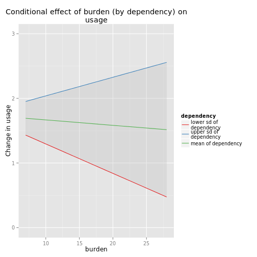
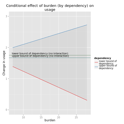
# plot interactions, including those with p-value up to 0.1
sjp.int(fit,
        type = "cond",
        plevel = 0.1,
        showInterceptLines = TRUE)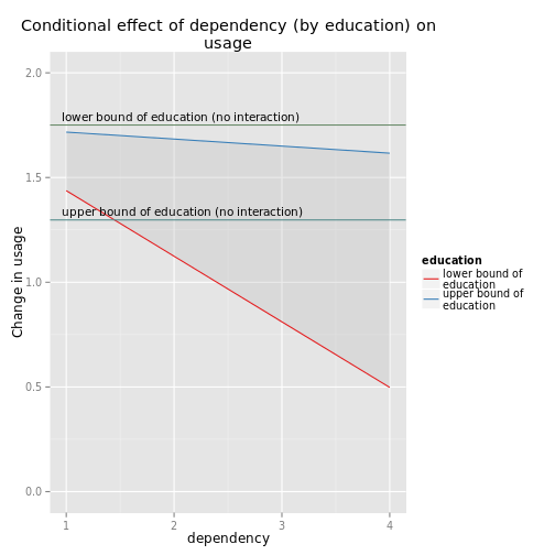
# -------------------------------
# Predictors for negative impact of care.
# Data from the EUROFAMCARE sample dataset
# -------------------------------
library(sjmisc)
data(efc)
# create binary response
y <- ifelse(efc$neg_c_7 < median(stats::na.omit(efc$neg_c_7)), 0, 1)
# create data frame for fitted model
mydf <- data.frame(y = as.factor(y),
                   sex = as.factor(efc$c161sex),
                   barthel = as.numeric(efc$barthtot))
# fit model
fit <- glm(y ~ sex * barthel,
           data = mydf,
           family = binomial(link = "logit"))
# plot interaction, increase p-level sensivity
sjp.int(fit,
        type = "eff",
        legendLabels = get_labels(efc$c161sex),
        plevel = 0.1)
## Error: Package 'effects' needed for this function to work. Please install it.sjp.int(fit,
type = "cond",
legendLabels = get_labels(efc$c161sex),
plevel = 0.1)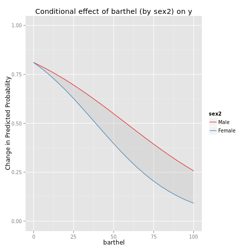
## Not run:
##D # -------------------------------
##D # Plot estimated marginal means
##D # -------------------------------
##D # load sample data set
##D library(sjmisc)
##D data(efc)
##D # create data frame with variables that should be included
##D # in the model
##D mydf <- data.frame(burden = efc$neg_c_7,
##D                    sex = efc$c161sex,
##D                    education = efc$c172code)
##D # convert gender predictor to factor
##D mydf$sex <- factor(mydf$sex)
##D mydf$education <- factor(mydf$education)
##D # name factor levels and dependent variable
##D levels(mydf$sex) <- c("female", "male")
##D levels(mydf$education) <- c("low", "mid", "high")
##D mydf$burden <- set_label(mydf$burden, "care burden")
##D # fit "dummy" model
##D fit <- lm(burden ~ .*., data = mydf)
##D summary(fit)
##D
##D # plot marginal means of interactions, no interaction found
##D sjp.int(fit, type = "emm")
##D # plot marginal means of interactions, including those with p-value up to 1
##D sjp.int(fit, type = "emm", plevel = 1)
##D # swap predictors
##D sjp.int(fit,
##D         type = "emm",
##D         plevel = 1,
##D         swapPredictors = TRUE)
##D
##D # -------------------------------
##D # Plot effects
##D # -------------------------------
##D # add continuous variable
##D mydf$barthel <- efc$barthtot
##D # re-fit model with continuous variable
##D fit <- lm(burden ~ .*., data = mydf)
##D
##D # plot effects
##D sjp.int(fit, type = "eff", showCI = TRUE)
##D
##D # plot effects, faceted
##D sjp.int(fit,
##D         type = "eff",
##D         int.plot.index = 3,
##D         showCI = TRUE,
##D         facet.grid = TRUE)
## End(Not run)